1. Introduction
Saiga antelope (Saiga tatarica) is a migratory steppe ungulate whose conservation status has improved substantially after severe historical declines, while its mobility, aggregation behaviour, disease sensitivity, and very large range continue to demand repeatable monitoring [1–7]. The species is particularly important in Kazakhstan because the country contains the dominant populations and the principal contemporary monitoring challenge: animals can occur in dense calving aggregations, move across broad landscapes, cross administrative boundaries, and change their apparent visual signature with season, illumination, dust, snow, and coat condition.
Aerial imagery offers scale and repeatability, but scale does not automatically produce biological validity. A frame can contain many visible animals while still failing to resolve the nasal profile, horns, limbs, or boundaries between neighbouring individuals. Conversely, an image can have a high nominal pixel count but poor ground sampling because sensor width, focal length, altitude, vibration, atmospheric path, compression, and exposure interact. The central problem is therefore not simply whether a model detects an animal. It is whether the complete observation system can support a specified scientific claim with measured uncertainty.
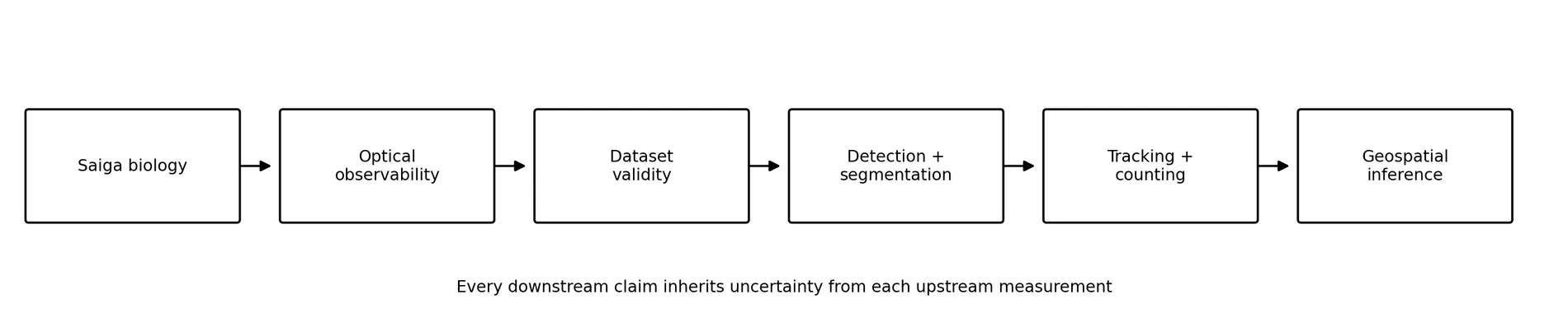
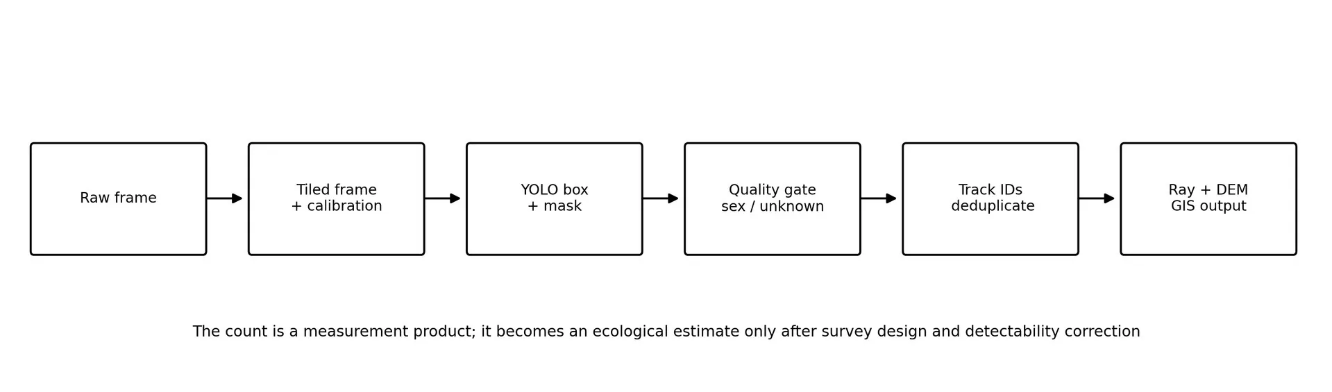
The framework follows the chain in Figure 1. Biological knowledge defines what counts as Saiga and what evidence can support sex assignment. Optical physics defines whether those features are observable. Dataset engineering determines whether the model is tested on genuinely independent conditions. Detection and segmentation produce visible-object measurements. Tracking removes repeated observations. Geospatial geometry maps observations to the ground. Survey design determines whether detections can be expanded to an abundance or distribution estimate.
1.1. Conservation context and monitoring need
The Saiga has an unusual conservation trajectory. The species experienced rapid losses associated with poaching, habitat pressures, disease, and mass mortality events, including the 2015 Kazakhstan die-off in which more than 200,000 animals died within approximately three weeks [5,6]. The later recovery that motivated the IUCN down-listing to Near Threatened is scientifically encouraging, but recovery changes the monitoring problem rather than eliminating it. Larger populations generate larger aggregations, wider movement footprints, more interactions with infrastructure and agriculture, and a greater need for comparable annual estimates [3,4].
Monitoring must consequently identify both ordinary population structure and abnormal conditions. The same georeferenced imagery that supports counts can also document unusual concentrations, mortality clusters, calving distribution, corridor use, or separation of herds across administrative and ecological boundaries. Those uses require a stable measurement protocol, not an opaque model whose training data, calibration, thresholds, and split logic cannot be audited.
1.2. Biological identity and the Saiga shape
Saiga identification should be based on morphology before colour. The most distinctive structure is the enlarged, flexible nasal vestibulum, which gives the head a short-trunk profile and supports physiological and acoustic adaptations described in detailed anatomical studies [2]. From an aerial viewpoint, species evidence is distributed across the head shape, body proportions, dorsal contour, leg arrangement, gait, pose, and ecological context. Coat colour is supporting evidence only because apparent colour changes with season, dust, snow, sun angle, white balance, exposure, and camera processing.
Sex identification is a separate task. Adult males usually show horns, whereas adult females are hornless. Horn visibility depends on head orientation, occlusion, pixel density, blur, and contrast. The nasal form of an adult male can provide secondary information in close, high-resolution imagery, but it should not substitute for horn evidence when the head is unresolved. Juveniles, distant individuals, side-on poses, and occluded heads must therefore be allowed to remain unknown rather than being forced into male or female classes.
The operational label ontology is consequently three-valued: sex ∈ {male, female, unknown}. The unknown state is not a failure of the method. It is a measurement statement that the image does not contain enough resolved evidence for a responsible classification. Treating unknown as a valid outcome prevents demographic bias caused by assigning every difficult animal to the nearest confident class.
sex ∈ {male, female, unknown} (Eq. 1)
1.3. Kazakhstan population systems and administrative geography
The CMS Saiga work programme distinguishes three principal Kazakhstan-linked population systems: Ural, Betpak-Dala, and Ustyurt [3]. These systems are ecological and management strata, not substitutes for administrative oblasts. The Ural system is associated with western Kazakhstan and transboundary movement toward Russia. Betpak-Dala occupies central Kazakhstan. Ustyurt is associated with the plateau west of the Aral Sea and transboundary context with Uzbekistan. The distinction matters because a population system describes biological connectivity, whereas an oblast describes governance and reporting jurisdiction.
| Population system | Geographic interpretation | Analytical use |
|---|---|---|
| Ural | Western Kazakhstan; seasonal transboundary context with Russia | Migration, corridor, and cross-border monitoring |
| Betpak-Dala | Central Kazakhstan steppe system | Calving, mortality, abundance, and seasonal aggregation |
| Ustyurt | Western plateau; Kazakhstan–Uzbekistan context | Distribution, movement, and sparse-landscape detection |
Table 1. Kazakhstan Saiga population systems used as ecological and management strata.
A detected animal should not be assigned to a region by visual approximation. The preferred procedure is to estimate a ground coordinate from calibrated camera pose, terrain elevation, and a viewing ray; then apply a versioned GIS point-in-polygon operation. The result can include population system, oblast, district, protected area, corridor, and survey stratum as separate attributes. This preserves the distinction between ecology, administration, and sampling design.
animal coordinate → versioned GIS point-in-polygon
    → {population system, oblast, district, corridor}                 (Eq. 2)
1.4. Objective and scope
The objective is to define a reproducible and critic-resistant framework for detecting, segmenting, sex-classifying, tracking, counting, and geolocating Saiga from aerial imagery in Kazakhstan. The scope includes the observation physics and information technology required to make those tasks auditable. It does not claim a field accuracy, abundance, sex ratio, or migration result without a measured dataset and a completed validation experiment. Analytical examples are explicitly labelled as examples so that numerical illustrations cannot be mistaken for empirical findings.
2. Research questions and hypotheses
The paper treats the monitoring system as a sequence of testable questions rather than as a single model benchmark. The questions determine which data must be collected and which error source must be isolated.
- RQ1. At what ground sampling distance and head/horn pixel density can experts and models distinguish Saiga from hard negative steppe objects?
- RQ2. How do altitude, focal length, exposure, motion blur, atmospheric path, and compression alter detection and segmentation quality?
- RQ3. Under what image-quality conditions can adult sex be assigned without introducing systematic class or geography bias?
- RQ4. How much do grouped flight, herd, date, and geographic splits change performance relative to random frame splits?
- RQ5. How accurately can a calibrated camera ray and terrain model place observations into Kazakhstan's ecological and administrative strata?
- RQ6. What is the difference between a visible-animal count in sampled imagery and a defensible abundance estimate for the population?
The primary hypotheses are that performance decreases as feature pixels and signal-to-noise ratio decline; that grouped geographic and encounter-level splits yield more conservative generalization estimates than random frame splits; that an unknown sex class improves calibration and reduces demographic bias; and that abundance inference requires detectability and sampling corrections that cannot be replaced by a neural-network confidence score.
3. Historical development of Saiga counting as a metrological system
3.1. The measurand: what does ‘the number of Saigas’ mean?
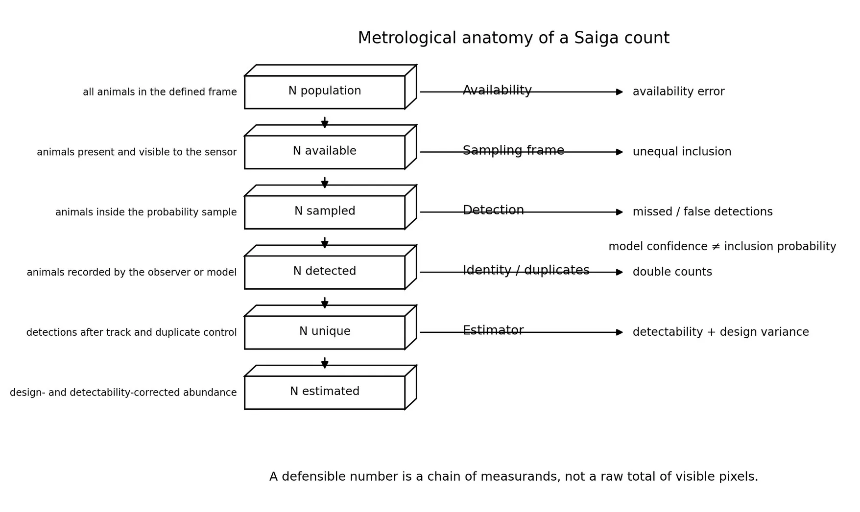
A count is not a single object that becomes more accurate simply because the camera becomes newer. It is a measurand: a defined quantity, observed under a specified protocol, with a stated relationship to the underlying population. In Saiga monitoring, at least six quantities can be confused: the population present in a region, the animals available to the observer, the animals included by the sampling design, the animals detected in imagery, the unique animals remaining after duplicate control, and the abundance estimate obtained after detectability correction.
The practical consequence is that two surveys can both be called ‘a census’ while measuring different quantities. A winter route may measure tracks or carcasses; an aircraft strip may measure visible groups within a sampled footprint; a UAS mission may measure unique detections during a short encounter; a design-based estimator may infer animals that were not visible in any one frame. Comparisons through time are meaningful only when the estimand, seasonal window, spatial frame, and correction logic are documented alongside the reported number [1,3,23,24].
E[N_detected] = N_population × p_available × p_sample × p_detect (Eq. M1)
Equation M1 is a conceptual factorisation, not a claim that every study must estimate each term independently. It makes the hidden assumptions visible: an animal can be absent from the sampled stratum, present but unavailable to the sensor, available but missed, or detected more than once. The visible total is therefore a conditional observation, whereas the abundance estimate is a model-based statement about the population that generated that observation.
N_estimated = g(N_unique, p_detect, p_available, π_i, design) (Eq. M2)
The symbol g in Eq. M2 represents the estimator appropriate to the survey design. The inclusion probability π_i and the detection model are not interchangeable with a detector confidence score. This distinction gives the paper its central viewpoint: technological progress is valuable when it makes one of these terms more measurable, not merely when it increases a benchmark score.
3.2. From field observation to organised census
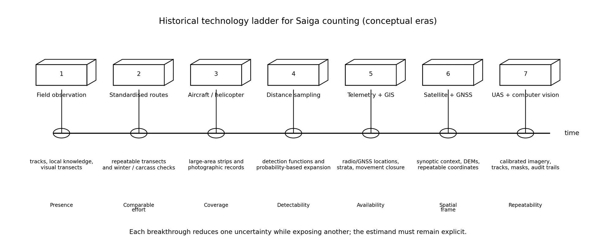
The earliest layer of Saiga monitoring is field observation: people follow routes, record sightings, interpret tracks, locate carcasses, and use local knowledge of seasonal movements. These observations are indispensable for discovering where animals are and when they aggregate, but they rarely provide an explicit probability of detection. A missed animal and an absent animal can look identical in the notebook. The historical value of these methods is therefore continuity and ecological context, not a false impression of complete enumeration.
The next step is standardised effort. Repeatable transects, fixed observation windows, winter or mortality checks, and shared reporting forms make counts comparable across years and teams. The improvement is metrological: the observation procedure becomes a documented instrument. Yet the main uncertainty remains visibility. Weather, observer fatigue, herd density, and animal movement can still change the number recorded even when the population is unchanged [1,24].
The timeline in Figure 6 is a history of measurement capability rather than a claim that one method replaced another on a single date. Current Kazakhstan monitoring still benefits from field observations, local expertise, and carcass investigations; the later technologies add scale and auditability rather than making those forms of evidence obsolete. The CMS work programme places monitoring, distribution, and temporal movement in the same conservation system, which is consistent with a layered rather than a single-sensor history [3,23].
3.3. Aerial surveys, distance sampling, and explicit detectability
Aircraft and helicopters changed the scale of the sampling frame. A survey team could move across broad steppe, follow planned strips, photograph aggregations, and revisit a route without relying entirely on ground access. The new failure modes were geometric and operational: strip width, altitude, image overlap, observer fatigue, aircraft motion, and repeated views of the same herd. A large visible total could still be biased if the flight path sampled some habitats or aggregations more often than others.
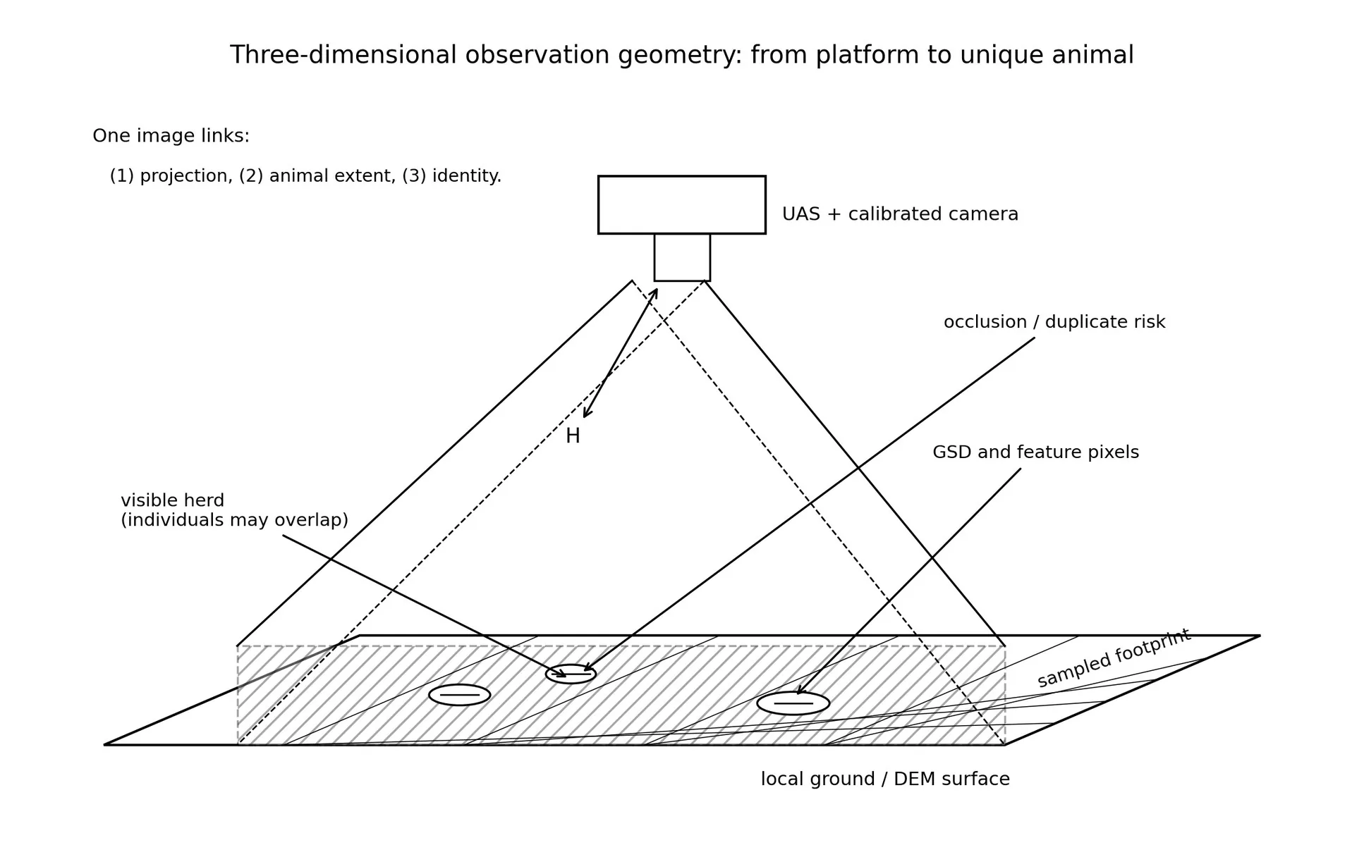
Distance sampling made the hidden term explicit by modelling how detection changes with distance from a transect line [17]. The method does not require every animal to be seen; it requires a defensible detection function, a defined sampling unit, and assumptions about distances, availability, and independence. For Saiga, the geometry is three-dimensional because camera rays meet uneven terrain and because a herd is a moving, partially occluded set of individuals. Figure 7 links these geometries to the count ledger.
The key historical shift is from ‘how many animals did the observer see?’ to ‘what sampling and detection process could have produced this observation?’ That shift is the bridge between natural-history observation and modern abundance estimation. It also explains why a detector can be accurate at the object level while the survey remains biased at the population level.
3.4. Telemetry, GNSS, GIS, and the separation of availability from detectability
Radio telemetry and later GNSS collars introduced a second kind of evidence: repeated locations of known individuals. These data do not directly count every Saiga, but they reveal movement timing, habitat use, corridor crossing, and the probability that animals are present within or outside a survey frame. In metrological terms, telemetry helps estimate availability and informs stratification; it does not replace the detection model for unmarked animals.
GIS made the separation operational. A camera ray or a telemetry fix can be assigned to an ecological population system, administrative district, protected area, or corridor only after the coordinate reference system, terrain model, and polygon version are recorded. This prevents a common historical mistake: treating a visually estimated location or a broad map label as if it were a measured boundary crossing. Coordinate uncertainty must be carried into the assignment, especially near borders and narrow corridors [3,20,21,23].
The parallel development is important. Better positioning does not automatically produce better abundance. GNSS can make the platform location precise while the animal remains ambiguous in the image; telemetry can show where collared animals travel while uncollared animals remain under-sampled. The technology reduces positional uncertainty and improves the sampling frame, but detectability and identity still require independent validation.
3.5. Drones, calibrated sensors, and computer vision
Unmanned aerial systems brought the camera closer to the scale of individual animals while retaining repeatable flight planning. A calibrated UAS frame can preserve image time, pose, overlap, terrain context, and an auditable chain from raw pixels to a detection. Computer vision then automates part of the transcription: boxes and masks locate visible animals, trackers link observations, and a GIS layer stores coordinates and uncertainty. The gain is repeatability and throughput, not automatic truth.
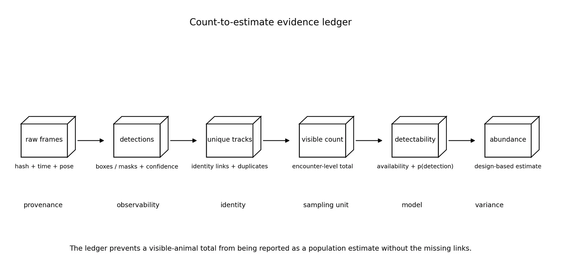
The new risks are correspondingly specific. A model may mistake livestock, shrubs, shadows, or snow for Saiga; segmentation can split or merge animals; track association can duplicate a herd; and a high-confidence prediction can still represent an animal outside the intended sampling unit. The evidence ledger in Figure 9 makes the missing links visible. A raw frame becomes a defensible abundance statement only when provenance, observability, identity, and survey design are all present.
3.6. Technology breakthroughs and the remaining uncertainty budget
Figure 8 summarises the paper’s point of view. Technologies do not simply move the entire error bar downward; they redistribute uncertainty. Aerial platforms reduce coverage uncertainty but expose strip-width and duplicate-encounter problems. Distance sampling formalises detectability but depends on its assumptions. Telemetry and GNSS improve availability and spatial frame definition but do not identify every unmarked animal. UAS and computer vision improve repeatability and throughput while introducing learned-model, calibration, and identity errors.
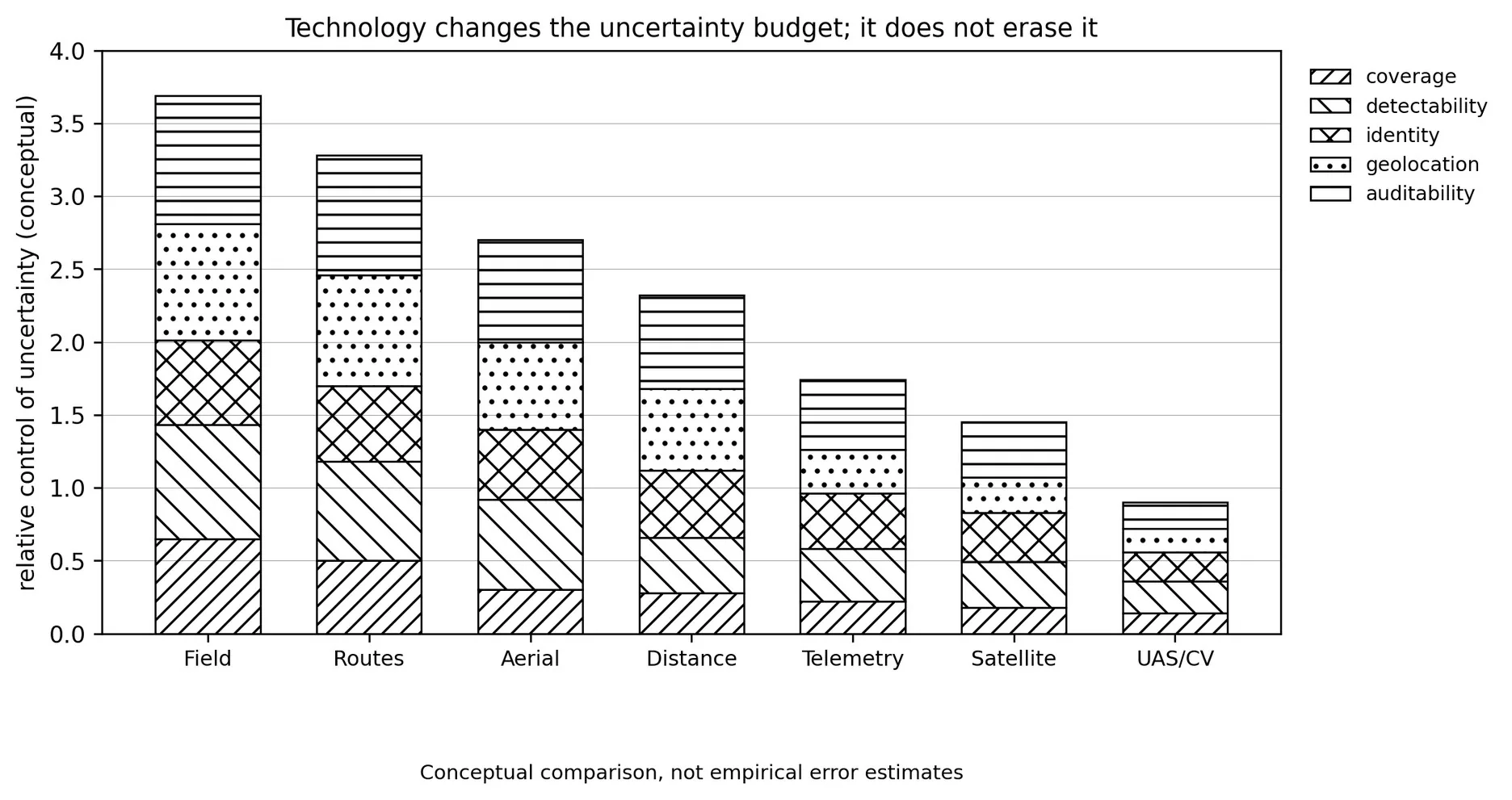
This history changes how a monitoring programme should define progress. A new camera or model is a scientific improvement only when it lowers a named uncertainty, makes a previously hidden assumption testable, or creates a better audit trail. The appropriate comparison is therefore not ‘old versus new device’ but ‘old versus new measurand chain’. With that historical and metrological context established, the next section develops the optical and statistical equations that govern the present aerial system.
4. Theoretical foundation
4.1. Observation as an inverse problem
A camera records a two-dimensional projection of a three-dimensional animal and its environment. The inverse problem is underdetermined: many combinations of distance, pose, terrain, illumination, and animal morphology can produce similar pixels. Scientific validity therefore depends on constraining the inverse problem with calibration, known geometry, biological priors, and explicit uncertainty.
s p = K [R | t] P (Eq. 3)
In Eq. 3, P is a point in world coordinates, p is its image coordinate, K contains intrinsic parameters such as focal length and principal point, R and t describe camera orientation and position, and s is a projective scale. Camera calibration using repeated views of a known target follows the flexible planar method of Zhang [10]. Without calibration, pixel measurements may still support qualitative detection, but high-accuracy ground coordinates are not justified.
4.2. Imaging physics: resolution, altitude, distance, brightness, and motion
Figure 10 summarizes the geometry. The camera height above local ground, physical sensor width, focal length, and image width jointly determine nominal ground sampling distance. Megapixels alone do not specify spatial resolution because two cameras with the same pixel count can have different sensor dimensions and focal lengths.
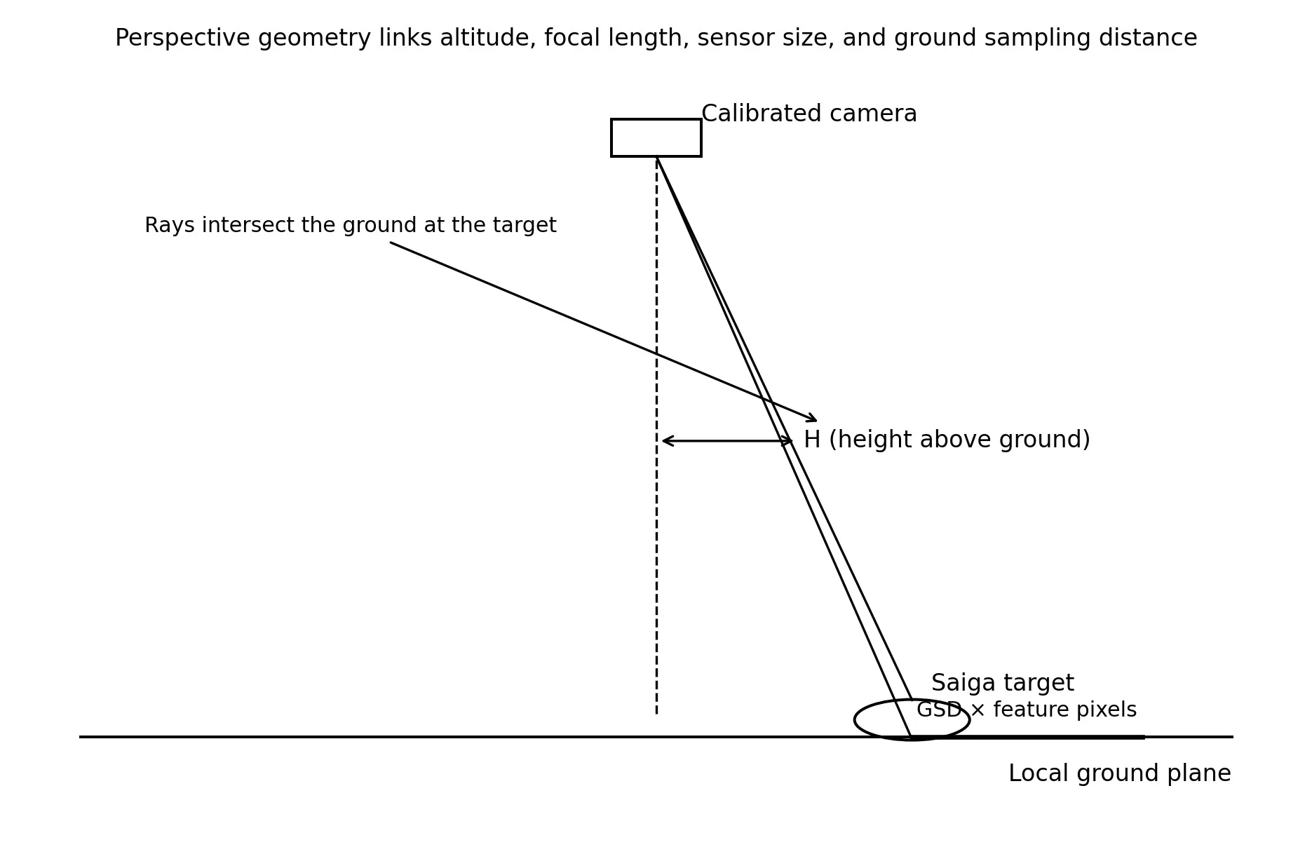
GSD_x = H · S_x / (f · N_x) (Eq. 4)
Here H is camera height above local ground, S_x is physical sensor width, f is focal length, and N_x is horizontal image width. A feature of physical size D occupies approximately:
n_px = D / GSD_x = D · f · N_x / (H · S_x) (Eq. 5)
For a prevalidated minimum feature resolution n_min, the maximum theoretical height is:
H_max = D · f · N_x / (n_min · S_x) (Eq. 6)
The word prevalidated is essential. A universal statement such as ‘Saiga can be detected at 120 m’ is not scientifically meaningful without the camera, lens, sensor, animal size, view angle, blur, image-processing path, and task definition. Detection, species discrimination, and horn-level sex assignment require progressively more information in the usual case.
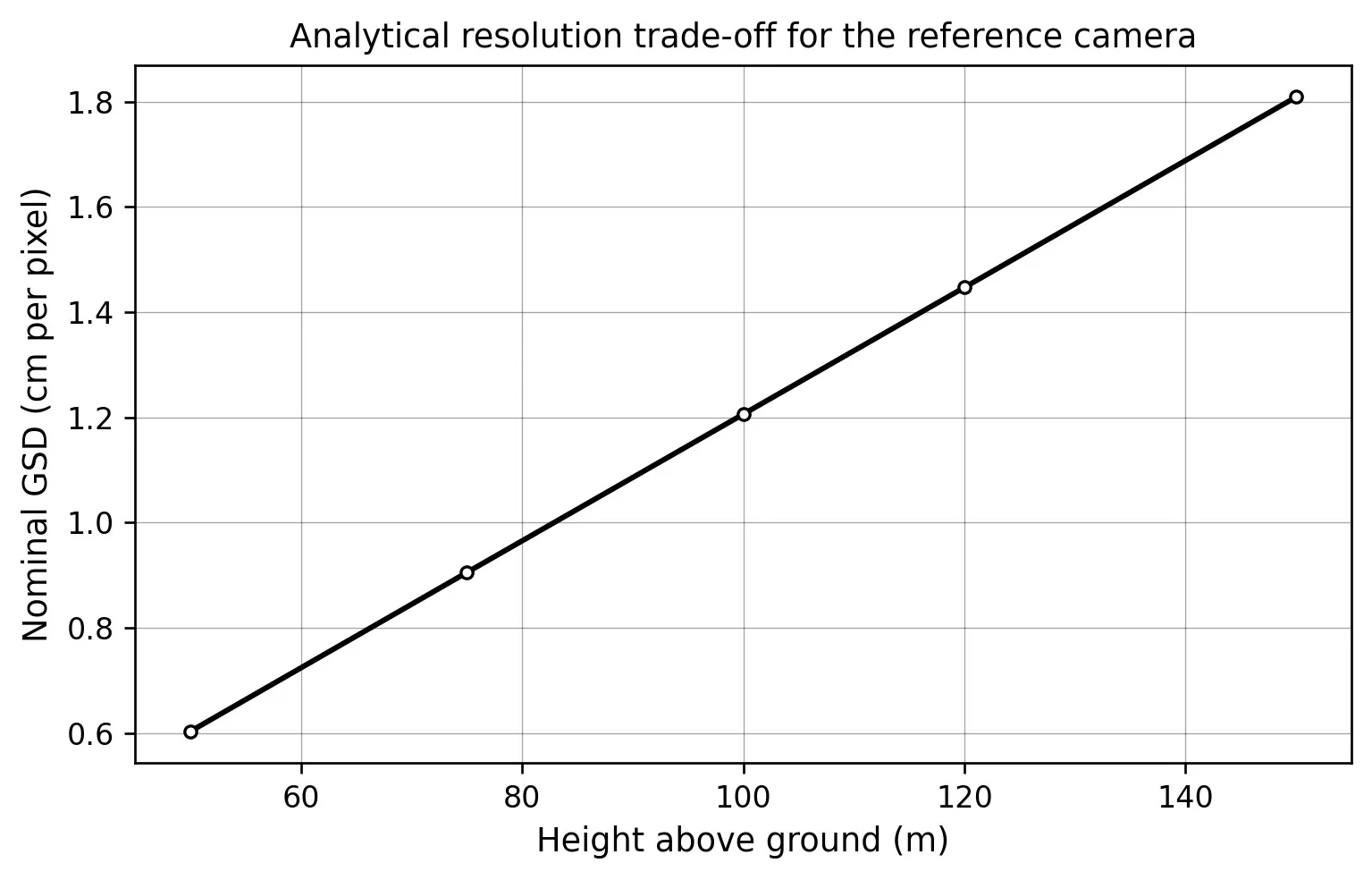
| Height AGL | Nominal GSD | Ground width | Pixels on 1 m feature | Pixels on 0.20 m feature |
|---|---|---|---|---|
| 50 m | 0.603 cm/px | 33.0 m | 165.8 | 33.2 |
| 75 m | 0.905 cm/px | 49.5 m | 110.5 | 22.1 |
| 100 m | 1.206 cm/px | 66.0 m | 82.9 | 16.6 |
| 120 m | 1.447 cm/px | 79.2 m | 69.1 | 13.8 |
| 150 m | 1.809 cm/px | 99.0 m | 55.3 | 11.1 |
Table 2. Analytical resolution example for S_x = 13.2 mm, f = 20 mm, and N_x = 5472 pixels. Values illustrate geometry and are not field performance claims.
4.3. Distance estimation and geolocation uncertainty
Monocular known-size ranging can provide a rough distance estimate when a feature of known physical size is resolved. For Saiga, however, physical size varies with sex, age, posture, orientation, foreshortening, and individual condition. Ranging should therefore be a secondary check rather than the primary coordinate method.
Z ≈ f_px · D / d_px,    f_px = f · N_x / S_x                         (Eq. 7)
(σ_Z / Z)² ≈ (σ_f / f)² + (σ_D / D)² + (σ_d / d)²                   (Eq. 8)
The preferred geolocation method intersects a calibrated camera ray with a digital elevation model or a locally surveyed ground surface. Uncertainty should propagate from camera position, orientation, lens calibration, terrain elevation, rolling-shutter timing, image point selection, and animal extent. RTK or GNSS improves platform position; it does not by itself reveal the ground coordinate of an animal observed at an oblique ray.
4.4. Brightness, signal-to-noise ratio, and motion blur
A common but incomplete argument is that an extended animal must become four times darker whenever range doubles. For a resolved extended target under fixed atmospheric and exposure conditions, scene radiance is the more relevant quantity than point-source inverse-square irradiance. Increasing range primarily reduces angular size and therefore the number of pixels assigned to the animal. Recorded brightness can nevertheless change because of atmospheric attenuation, haze, exposure automation, vignetting, optical transmission, sun geometry, reflectance, and compression.
E_image ∝ L_scene · t / N_f²                                         (Eq. 9)
SNR ≈ N_s / √(N_s + N_b + σ_r²)                                      (Eq. 10)
In Eq. 9, L_scene is scene radiance, t is exposure time, and N_f is f-number. In Eq. 10, N_s is signal electrons, N_b is background electrons, and σ_r is read noise. Increasing exposure can improve photon statistics but also increases motion blur. For relative ground speed v_rel, a first-order blur estimate is:
b_px ≈ v_rel · t / GSD                                                (Eq. 11)
t_max ≈ b_max · GSD / v_rel                                           (Eq. 12)
The effective point-spread function is the combined result of pixel sampling, lens aberration, diffraction, defocus, vibration, motion, rolling shutter, atmospheric turbulence, demosaicing, compression, and resizing. A defensible flight protocol must measure or bound the dominant terms instead of treating nominal camera resolution as a complete description of image quality.
| Variable | Physical effect | Measurement control |
|---|---|---|
| Altitude | Changes GSD and target angular size | Record AGL and terrain-relative height |
| Focal length | Changes angular magnification and field of view | Archive calibrated lens state |
| Exposure time | Controls photon collection and motion blur | Record shutter, ISO, aperture, and blur proxy |
| Atmosphere | Attenuates contrast and adds haze | Record visibility, sun angle, and weather |
| Compression | Removes fine boundaries and texture | Preserve original files and codec metadata |
Table 3. Variables that alter biological observability even when nominal pixel count is unchanged.
5. Materials and methods
5.1. Study design and unit of analysis
The study is designed as a hierarchical observational experiment. The primary acquisition unit is a flight or transect. Within a flight, frames are correlated because they view the same terrain, herd, and illumination. Within a herd encounter, adjacent frames are not independent animals. Splits and statistical uncertainty must therefore be clustered at the flight, encounter, date, and geographic level rather than treating every frame as an independent sample.
The protocol has two phases. Phase A measures observability and builds the dataset. Phase B locks the dataset, model configuration, and evaluation code before the final test is opened. Any change to labels, split membership, calibration, or model configuration after test inspection creates a new experiment and must be recorded as such.
5.2. Data acquisition and dataset curation
Raw imagery should be captured in the original camera format when feasible, with the aircraft position, attitude, lens state, exposure, timestamp, frame identifier, and weather metadata retained. Every file receives a cryptographic hash. The manifest links each frame to its flight, herd encounter, date, geographic stratum, sensor configuration, and annotation version. Precise wildlife locations should be access-controlled because publishing them can increase poaching risk.
Annotations should distinguish visible body extent from truncated or occluded extent. Bounding boxes and instance masks should not imply certainty where animal boundaries are hidden. Each candidate receives species status, visibility quality, adult or juvenile status when justified, sex label or unknown, occlusion, truncation, pose, and annotation confidence. Double annotation and adjudication are required for the test set. The adjudication record should preserve the original labels and the reason for each resolution.
| Stratum | Examples | Purpose |
|---|---|---|
| Geography | Ural, Betpak-Dala, Ustyurt; oblast and district | Test geographic transfer and GIS attribution |
| Season | Calving, summer, autumn, winter | Test coat, aggregation, and illumination changes |
| Object scale | Small, medium, large image extent | Measure resolution dependence |
| Scene context | Empty steppe, livestock, vehicles, shrubs, snow | Measure hard-negative false positives |
| Visibility | Clear, occluded, truncated, motion blurred | Support quality-gated inference |
Table 4. Minimum dataset strata required before a headline test metric can be interpreted as generalization.
The recommended split is grouped by flight, herd encounter, date, and spatial block. A random frame split is retained only as a diagnostic because it can place near-duplicate frames from one encounter in both training and test sets. An external geographic holdout is the strongest available test of transfer within Kazakhstan. If the holdout is too small for stable estimates, that limitation is reported rather than hidden by pooling it into the main test set.
5.3. YOLO detection and instance segmentation
The YOLO family is used as an operational baseline because single-stage detectors can provide low-latency inference and modern implementations can expose detection, segmentation, tracking, and export paths [8,12,13]. The word YOLO does not identify a unique scientific method. The exact model generation, package version, pretrained checkpoint, weights hash, image size, optimizer, learning-rate schedule, augmentation policy, batch size, confidence threshold, intersection-over-union threshold, random seed, early-stopping rule, export runtime, and licence state must be archived.
A generic multi-task objective can be expressed as:
L_total = λ_box L_box + λ_cls L_cls + λ_mask L_mask + λ_aux L_aux (Eq. 13)
The symbols in Eq. 13 are intentionally generic because loss definitions and label assignment can change between model generations. The paper therefore treats the equation as an accounting structure, not as a claim that all implementations use identical losses. An independent segmentation baseline such as Mask R-CNN [9] is required for scientific comparison when mask quality is central. If both models fail on small or occluded animals, that is evidence about observability and data quality rather than proof that one brand of architecture is universally inadequate.
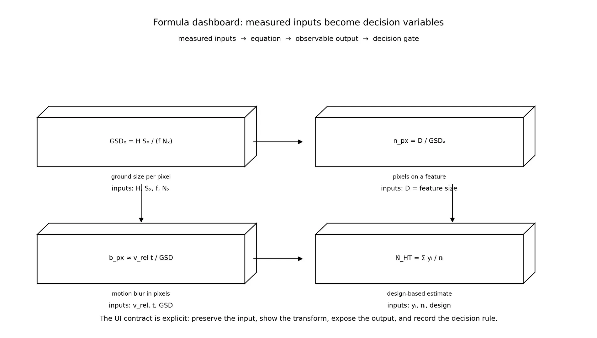
The equations are easier to implement when they are treated as user-interface contracts rather than isolated lines of notation. Figure 13 therefore places each formula beside its measured inputs, its transformed quantity, and the decision it supports. This representation makes a missing calibration value or an unjustified inference visible before the result is exported.
5.4. Sex classification and abstention
Sex is assigned only when the image resolves evidence appropriate to the label. The annotation protocol records whether horns are visible, whether the head is sufficiently resolved, whether the animal is adult, and whether another animal or vegetation occludes the relevant anatomy. A classifier may output a probability distribution, but the final operational label is male, female, or unknown after a pre-registered quality gate.
Performance must be reported in two dimensions: conditional accuracy on eligible images and coverage, the fraction of eligible animals receiving a sex assignment. A system that assigns sex to only easy animals can have high conditional accuracy and poor scientific utility. The unknown class should therefore be reported by geography, season, scale, occlusion, and sex-reference availability.
coverage = N_sex-assigned / N_eligible Saiga (Eq. 14)
5.5. Tracking, counting, and deduplication
Object detection produces frame-level observations, not unique animals. Tracking links detections across frames using appearance, motion, time, and camera geometry. A simple online tracking baseline can be reported using a Kalman filter and assignment procedure [14,15], but the tracking configuration must be tested under herd density, occlusion, crossing trajectories, and camera motion.
Counting accuracy should be evaluated separately from detection accuracy. The count for a frame or encounter is affected by false positives, missed animals, overlapping masks, truncation, track fragmentation, and duplicate tracks. Manual review of a stratified subset of tracks should estimate identity switches and duplicate rates. The result is a sampled visible-animal count, not automatically a population abundance estimate.
MAE_count = (1/n) Σ_j |ĉ_j − c_j| (Eq. 15)
5.6. Geolocation and GIS attribution
The geolocation workflow stores both the estimated animal coordinate and the uncertainty ellipse or covariance representation. The coordinate is produced by intersecting the camera ray with the terrain model or a surveyed plane. Each output record retains camera intrinsics, camera pose, terrain model version, timestamp, frame identifier, detection identifier, and coordinate reference system.
GIS attribution is performed after coordinate estimation. Point-in-polygon operations assign population system, oblast, district, protected area, and corridor in separate fields. Boundary cases are flagged when coordinate uncertainty crosses a polygon edge. A field that appears precise to six decimal places is not necessarily accurate to six decimal places; the stored uncertainty must control the number of meaningful digits reported to users.
5.7. Statistical validation and ecological inference
Detection evaluation uses intersection over union, precision, recall, F1, and average precision across multiple overlap thresholds. Mask evaluation uses overlap metrics such as Dice and mask average precision. All metrics are reported with clustered confidence intervals or bootstrap resampling at the flight, encounter, or spatial-block level. Frame-level bootstrap intervals are not acceptable when frames are correlated.
IoU = |A ∩ B| / |A ∪ B|                                              (Eq. 16)
Precision = TP / (TP + FP),   Recall = TP / (TP + FN)               (Eq. 17)
F1 = 2PR / (P + R)                                                   (Eq. 18)
Dice = 2|M ∩ G| / (|M| + |G|)                                        (Eq. 19)
A survey estimate requires a sampling design and a detection model. For a probability sample, the Horvitz–Thompson estimator is:
N̂_HT = Σ_i y_i / π_i (Eq. 20)
The inclusion probability π_i is determined by the survey design and is not the same quantity as a model confidence score. Distance sampling, occupancy models, or spatial mark–recapture can be appropriate depending on the design and estimand [16–18]. A detector can be excellent while an abundance estimate remains biased if animals are unavailable, hidden, clustered, or sampled with unequal probability.
5.8. Information technology and reproducibility controls
The computational record must be sufficient for an independent group to reconstruct the result. The minimum archive includes raw-frame hashes, annotation version, split manifest, camera calibration, terrain model, model configuration, weight hash, training seed, software environment, hardware description, evaluation thresholds, and exported prediction files. The archive should also record failed runs and exclusion decisions because selective reporting can make a system appear more stable than it is.
The data model should treat each prediction as an auditable record rather than a detached image overlay. A recommended record contains frame hash, flight identifier, timestamp, geographic stratum, detector version, mask geometry, confidence, quality gate, sex state, track identifier, coordinate, uncertainty, and processing status. Hashes follow the Secure Hash Standard [22]. Spatial data should use a versioned coordinate reference system and a documented GIS data-quality procedure [20,21].
6. Technical implementation and validation results
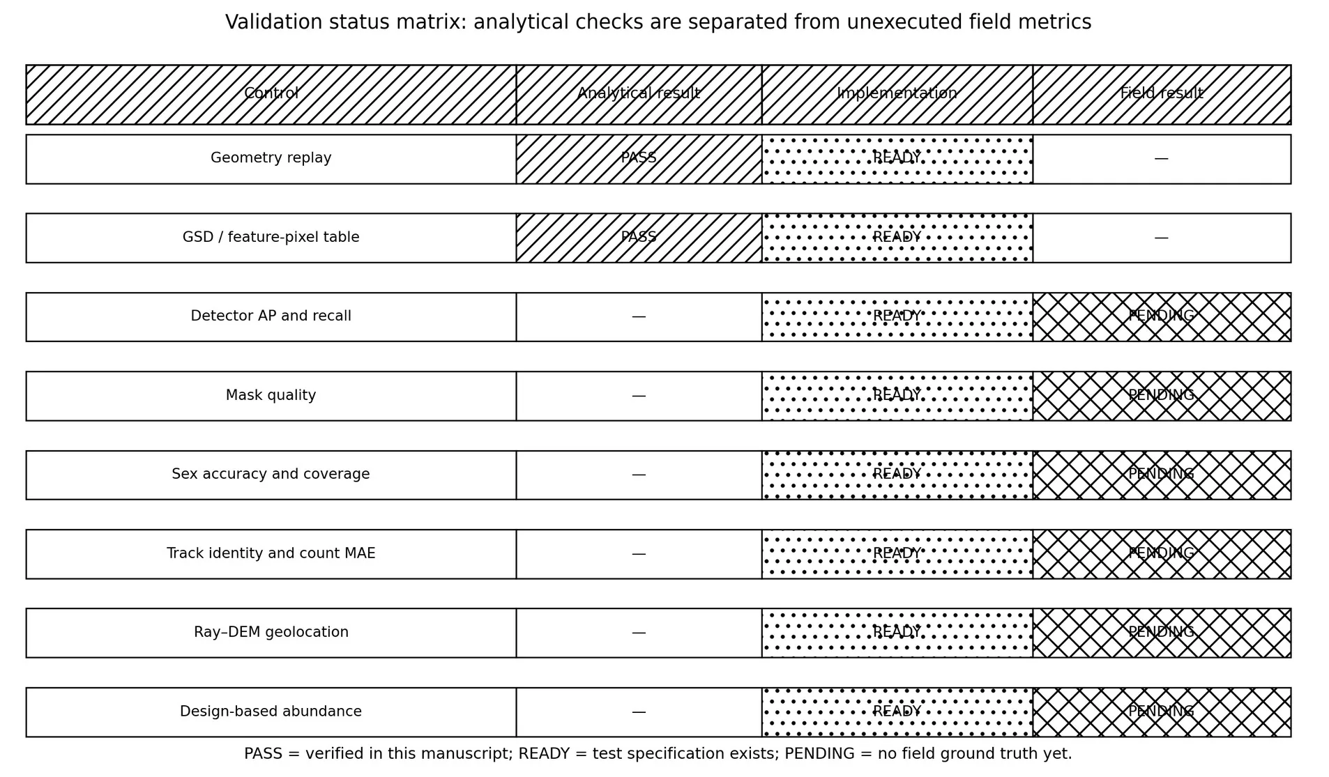
The proposed method becomes testable only when the biological claim, software stack, measurement inputs, and acceptance rule are written together. This section therefore separates three result levels: an analytical result that can be checked from the equations, an implementation result that can be reproduced from the recorded stack, and an empirical field result that requires locked imagery and independent ground truth. Only the first two levels are available in the present manuscript; no field accuracy, abundance, sex ratio, or disturbance result is invented.
6.1. Reference implementation stack
The following stack is the reference implementation configuration for a reproducible pilot. It is deliberately modular: the detector can be replaced without changing the camera calibration, tracking ledger, GIS attribution, or survey estimator. Configuration values such as image size, epochs, and batch size are baseline settings to be tested, not evidence that one training run is optimal.
| Layer | Reference implementation | Reproducibility record |
|---|---|---|
| Flight data | UAV RGB with optional thermal payload; calibrated intrinsics and extrinsics; RTK/GNSS; target 2–5 cm GSD and more than one hour endurance for broad transects | Original media, flight log, pose/time manifest, camera profile, weather |
| Annotation | CVAT with YOLO and COCO export; visible masks, occlusion and truncation, adult/juvenile status, male/female/unknown metadata | Immutable label version, adjudication log, label hashes |
| Detector | Ultralytics YOLO11; yolo11s.pt baseline; Python 3.12.3; PyTorch CUDA wheel; imgsz 1280; batch 32; 100-epoch ceiling | Package and checkpoint versions, weights hash, seed, configuration, licence state |
| Segmenter | Independent Mask R-CNN baseline so mask quality is not judged only by the detector family | Model configuration, weights hash, mask metrics |
| Tracking | ByteTrack or OC-SORT with Kalman association and spatiotemporal deduplication | Tracker parameters, identity-switch log, track manifest |
| Geospatial | OpenCV calibration; GDAL, GeoPandas, and QGIS; digital elevation model; versioned CRS and point-in-polygon operations | Intrinsics/extrinsics, DEM hash, CRS, ray uncertainty, polygon version |
| Data and provenance | DVC with S3 or MinIO object storage; Parquet or CSV prediction ledger; SHA-256 file hashes | Train/validation/test manifests, environment lockfile, run metadata |
| Compute | Dual NVIDIA H100 NVL development node; GPU 0 reserved; driver 570.172.08 with CUDA 12.8 compatibility | Hardware description, driver, container or environment export |
Table 7. Reference implementation stack and the record required for reproducibility.
The detector is intentionally treated as a versioned component rather than as the definition of the method. A replacement model is acceptable only when it is evaluated on the same grouped split, receives the same calibration and sampling metadata, and produces an auditable prediction ledger. Ultralytics licensing is a deployment parameter and must be recorded with the selected package and export runtime.
6.2. Technical test protocol
The test sequence follows the measurement chain. Geometry is tested before model training; dataset leakage is tested before headline metrics; detection and segmentation are tested before tracking; tracking is tested before counting; and abundance inference is attempted only after inclusion and detectability are specified. This ordering prevents a strong object-level score from masking a failure in the population-level claim.
| Test | Input and procedure | Output and decision rule |
|---|---|---|
| Geometry replay | Reference camera parameters and heights from 50–150 m; recompute GSD and feature pixels | Values must match Eq. 4–6 within a declared numerical tolerance |
| Leakage audit | Compare random-frame, grouped flight/herd/date, and spatial-block splits | Grouped estimate is primary; a large random-to-grouped gap is a leakage warning |
| Detector and segmenter | Locked test set with hard negatives and visible-mask labels | Box AP, recall, precision, mask AP, Dice, and clustered confidence intervals |
| Sex quality gate | Adult, head-resolved reference images stratified by geography, season, and scale | Male/female metrics, calibration, unknown coverage, and demographic balance |
| Track and count | Encounter-level sequences with manual identity review | Count MAE, MAPE, identity switches, fragmentation, and duplicate rate |
| Geolocation | Calibration targets, independent check points, ray–DEM intersection | Median and percentile error plus uncertainty-ellipse coverage |
| Abundance | Probability-based survey frame with availability and detection model | Estimator and sampling variance; no population claim if inclusion is undefined |
Table 8. Technical tests, inputs, outputs, and decision rules.
6.3. Verified analytical results
For the reference camera with sensor width 13.2 mm, focal length 20 mm, and image width 5472 pixels, the geometry calculation gives 0.603 cm per pixel at 50 m and 1.809 cm per pixel at 150 m. A 0.20 m feature therefore falls from approximately 33.2 pixels to 11.1 pixels across that height range. The positive result is internal consistency: the table, line plot, heatmap, and sensitivity chart all derive from the same equations. The negative result is the observability trade-off: higher coverage does not preserve fine morphology, so head and horn claims cannot be inferred from altitude alone.
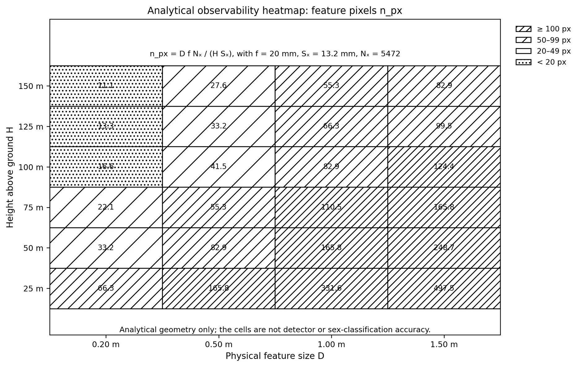
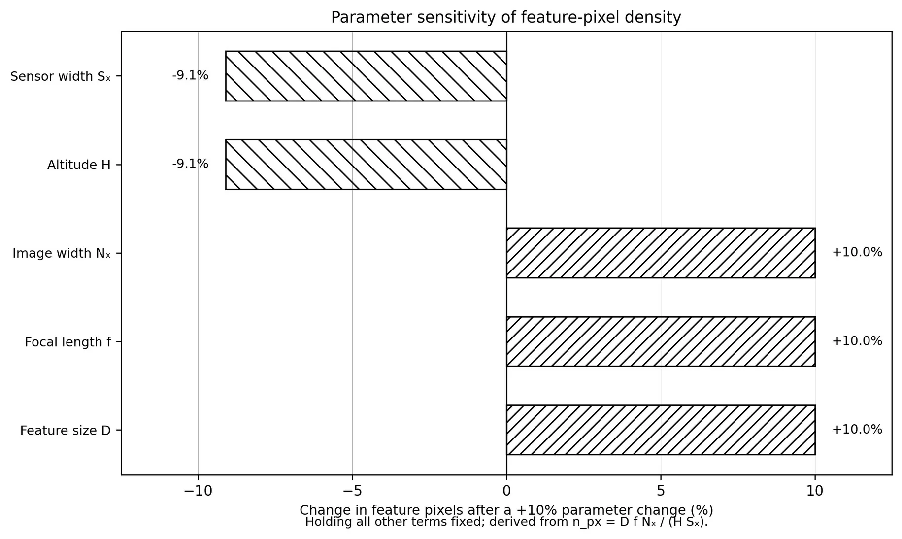
The charts expose a practical design rule. Feature size, focal length, and image width increase pixel evidence, whereas altitude and physical sensor width reduce it. The relationship is not a substitute for a field threshold because blur, atmosphere, pose, occlusion, and animal behaviour can remove information after the geometric calculation has passed.
6.4. Positive findings and implementation readiness
The present positive findings are limited but reproducible. They show that the proposed implementation has a coherent computational path and that its analytical claims can be checked without hidden model output.
| Finding | Status | Evidence and interpretation |
|---|---|---|
| GSD and feature-pixel replay | PASS | Reference values reproduce the stated equations at 50–150 m; this verifies geometry, not field detection |
| Monotonic altitude response | PASS | GSD increases and feature pixels decrease as height rises; the trade-off is visible in Figures 11 and 14 |
| Formula traceability | PASS | Figure 13 links inputs, transformations, outputs, and decision gates |
| Leakage-resistant evaluation design | READY | Grouped flight, herd, date, and spatial splits are specified before test opening |
| Reproducible software record | READY | Hashes, manifests, calibration, GIS versions, environment, and model configuration are defined |
Table 9. Positive analytical findings and implementation-readiness results.
6.5. Negative findings and unresolved risks
The negative findings are equally important because they define what the method cannot claim yet. ‘Pending’ does not mean that a model will fail; it means that the required ground truth and independent test have not been supplied. Reporting this boundary is preferable to filling it with plausible-looking metrics.
| Claim | Current status | Why the claim remains unresolved |
|---|---|---|
| Fine morphology at high altitude | NEGATIVE analytical constraint | A 0.20 m feature is only 11.1 pixels at 150 m; head and horn evidence cannot be assumed |
| Detector AP and recall | NOT MEASURED | No locked field test with independent hard-negative evaluation is included |
| Mask quality and occlusion | NOT MEASURED | No completed mask ground truth or boundary audit is reported |
| Sex accuracy and coverage | NOT MEASURED | No head-resolved adult reference set with geographic and seasonal balance is reported |
| Track identity and count error | NOT MEASURED | No manually reviewed encounter sequences are available for identity switches and duplicates |
| UAV disturbance and endurance | NOT MEASURED | No species-specific disturbance experiment or completed broad-transect flight log is included |
| Population abundance | BLOCKED | Inclusion, availability, and detectability are not empirically estimated |
Table 10. Negative or unresolved findings that block a biological performance claim.
6.6. Required empirical outputs
A completed field study should report results by the strata that determine transfer: geographic population system, season, object scale, visibility, and scene context. Each table should show encounters, animals, and frames; eligible sex labels; uncertainty intervals; and the evaluation threshold. A single pooled mAP value is insufficient because pooled metrics can conceal failure on small animals, empty steppe, or a population system absent from training data. Figure 16 provides the publication rule in one view: analytical passes and implementation readiness are not interchangeable with field results.
| Claim under review | Required evidence | Minimum reporting |
|---|---|---|
| Animal detection | Grouped test split and hard negatives | Precision, recall, AP at multiple IoU thresholds, false positives per km² or frame |
| Instance boundaries | Visible-mask annotation and occlusion labels | Mask AP, Dice, boundary errors, truncation analysis |
| Sex assignment | Adult, head-resolved reference labels | Male/female performance, unknown coverage, calibration |
| Unique counts | Track-level review and duplicate audit | Count MAE, track fragmentation, identity switches |
| Geolocation | Calibration, pose, terrain, independent check points | Median error, percentile error, uncertainty coverage |
| Population inference | Probability-based survey design | Estimator, detectability model, sampling variance |
Table 11. Evidence required before converting a model output into a biological or geographic claim.
7. Discussion
7.1. Why shape must precede colour
Saiga colour is a fragile feature because illumination, season, coat condition, dust, snow, and image processing alter the recorded RGB values. The flexible nasal structure and body geometry are more stable biological cues, although they also become unavailable when the animal is small, occluded, or blurred. A robust model should therefore learn shape, context, and texture jointly, while the annotation and validation protocol must make clear which visual evidence was actually resolved.
This principle also explains why a high-confidence prediction can be wrong. A model may associate a particular shade of steppe or a particular flight altitude with Saiga because the dataset contains geographic or seasonal shortcuts. Hard negatives, geographic holdouts, and deliberate changes in illumination are needed to test whether the model has learned the animal rather than the acquisition context.
7.2. Why height cannot be chosen by convention
Altitude is a multi-objective design variable. Lower altitude improves feature pixels and may improve head or horn resolution, but it reduces ground coverage, can increase motion and perspective variation, and may increase disturbance. Higher altitude covers more area and may reduce some disturbance risk, but it decreases pixels per animal and can reduce the signal-to-noise ratio after resizing. The chosen height must therefore satisfy a measured observability threshold, a disturbance assessment, weather and aviation constraints, and the survey design's coverage requirement.
A disturbance-free altitude cannot be borrowed from another species or aircraft without validation. Sound pressure, frequency content, flight path, speed, wind, habitat, herd state, and animal sensitivity all matter. The paper treats disturbance as a separate experiment and documents the behavioural indicators that would trigger a change in altitude, speed, route, or mission termination.
7.3. Dataset quality is a scientific variable
Dataset size is not a proxy for dataset quality. Ten thousand near-duplicate frames from one herd can be less informative than a smaller dataset that spans the three population systems, multiple seasons, illumination states, weather conditions, object scales, hard negatives, and independent flight encounters. Geographic and temporal diversity are especially important because Kazakhstan is not a single visual environment.
Leakage is the most common hidden inflation mechanism. If consecutive frames from one encounter are split randomly, the model can memorize background, pose, and herd-specific appearance. Grouped splits reduce this leakage. An external spatial holdout tests whether the learned representation transfers across regions. A serious manuscript reports both the random-frame diagnostic and the grouped estimate, explaining why the grouped estimate is the scientific result.
7.4. Epochs, models, and reproducibility
The number of training epochs is a ceiling, not a scientific result. A claim such as ‘200 epochs was optimal’ requires a convergence curve, validation protocol, early-stopping rule, random seed policy, and comparison against alternative ceilings. The same logic applies to model size, image size, augmentations, and confidence thresholds. Every selected setting must be tied to a locked validation procedure rather than to a single convenient run.
Model names also require version discipline. YOLO denotes a family of implementations, not a timeless algorithm. Reproducibility requires the exact package commit or release, configuration, pretrained weights, license, export path, and runtime. A future replacement can be scientifically valid, but it is a new model and must be reported as such.
7.5. What a critic can and cannot infer
| Potential criticism | Required defense |
|---|---|
| Training and test images are near duplicates | Grouped flight, herd, date, and spatial splits; external geographic holdout |
| Sex labels are guesses | Adult/head-resolution gate; male, female, and unknown ontology; adjudication log |
| Height was arbitrary | GSD, feature pixels, blur, SNR, disturbance, and regulatory derivation |
| Nominal megapixels prove resolution | Physical sensor size, focal length, altitude, and GSD calculation |
| The animal becomes four times darker at double range | Extended-target radiance, angular size, attenuation, exposure, and SNR analysis |
| RTK gives exact animal coordinates | Ray–terrain intersection and propagated camera, DEM, and image-point uncertainty |
| High AP proves population abundance | Separate detection, tracking, deduplication, sampling, and detectability models |
| A large dataset is automatically good | Diversity, hard negatives, geographic strata, and leakage testing |
| Drone altitude is harmless | Species-specific disturbance experiment and stop rules |
Table 6. Critic-resistant controls linking common objections to auditable evidence.
7.6. Limitations
The framework cannot remove information that is absent from an image. Severe occlusion, very small animals, fog, dust, motion blur, clipped highlights, and compression can make species or sex evidence unavailable. Unknown outputs and confidence intervals must remain visible in the final product. The framework also does not replace field verification, veterinary investigation, local ecological knowledge, or protected-area governance.
Geolocation uncertainty may be larger than the animal itself when terrain models are coarse or the camera is oblique. In dense herds, segmentation and tracking can fail jointly because one animal hides another and identities cross. Finally, a model trained in Kazakhstan can still fail on a new camera, new season, or new population system. External validation is not optional when the intended use is operational conservation.
8. Conclusions
A defensible Saiga monitoring system is a calibrated chain of biological, optical, computational, and ecological measurements. The Saiga's nasal profile and body form provide the biological basis for identification, while adult horns can support sex classification only when the head is resolved. Camera height, sensor dimensions, focal length, ground sampling distance, brightness, signal-to-noise ratio, and motion blur determine whether those features are observable. Dataset diversity, grouped splits, hard negatives, and an unknown sex state determine whether a model's performance is credible. Tracking and GIS geometry determine whether frame-level detections become unique, georeferenced observations. Survey design and detectability correction determine whether those observations support population inference.
The resulting framework is intentionally conservative. It reports analytical physics calculations as calculations, planned empirical outputs as planned outputs, and measured results only when a locked dataset and independent test make them available. That separation is the strongest protection against overclaiming. It also creates a clear implementation path: collect representative data, calibrate the camera, annotate morphology and uncertainty, train an explicitly versioned detector and segmentation model, validate by encounter and geography, propagate coordinate uncertainty, and publish the complete audit trail.
References
- Bekenov, A. B., Grachev, I. A., and Milner-Gulland, E. J. (1998). The ecology and management of the Saiga antelope in Kazakhstan. Mammal Review, 28, 1–52. https://doi.org/10.1046/j.1365-2907.1998.281024.x
- Frey, R., Volodin, I., and Volodina, E. (2007). A nose that roars: Anatomical specializations and behavioural features of rutting male saiga. Journal of Anatomy, 211, 717–736. https://doi.org/10.1111/j.1469-7580.2007.00818.x
- Convention on the Conservation of Migratory Species of Wild Animals. (2025). Medium-Term International Work Programme for the Saiga Antelope 2025–2030, UNEP/CMS/Saiga/MOS5/Outcome 2/Rev.1. https://saiga.cms.int/
- IUCN SSC Antelope Specialist Group. (2024). Saiga tatarica. The IUCN Red List of Threatened Species 2024: e.T19832A1983220242. https://doi.org/10.2305/IUCN.UK.2024-1.RLTS.T19832A1983220242.en
- Kock, R. A., Orynbayev, M., Robinson, S., Zuther, S., Singh, N. J., Beauvais, W., et al. (2018). Saigas on the brink: Multidisciplinary analysis of the factors influencing mass mortality events. Science Advances, 4, eaao2314. https://doi.org/10.1126/sciadv.aao2314
- Fereidouni, S., Orynbayev, M., Samy, A., et al. (2019). Mass die-off of Saiga antelopes, Kazakhstan, 2015. Emerging Infectious Diseases, 25, 1164–1172. https://doi.org/10.3201/eid2506.180990
- Orynbayev, M., Sultankulova, K., Sansyzbay, A., et al. (2019). Biological characterization of Pasteurella multocida present in the Saiga population. BMC Microbiology, 19, 37. https://doi.org/10.1186/s12866-019-1407-9
- Redmon, J., Divvala, S., Girshick, R., and Farhadi, A. (2016). You only look once: Unified, real-time object detection. Proceedings of the IEEE Conference on Computer Vision and Pattern Recognition, 779–788. https://doi.org/10.1109/CVPR.2016.91
- He, K., Gkioxari, G., Dollár, P., and Girshick, R. (2017). Mask R-CNN. Proceedings of the IEEE International Conference on Computer Vision, 2961–2969. https://doi.org/10.1109/ICCV.2017.322
- Zhang, Z. (2000). A flexible new technique for camera calibration. IEEE Transactions on Pattern Analysis and Machine Intelligence, 22, 1330–1334. https://doi.org/10.1109/34.888718
- Lin, T.-Y., Maire, M., Belongie, S., et al. (2014). Microsoft COCO: Common objects in context. In European Conference on Computer Vision, 740–755. https://doi.org/10.1007/978-3-319-10602-1_48
- Bochkovskiy, A., Wang, C.-Y., and Liao, H.-Y. M. (2020). YOLOv4: Optimal speed and accuracy of object detection. arXiv:2004.10934. https://arxiv.org/abs/2004.10934
- Ultralytics. (2026). Ultralytics YOLO documentation: Detection, segmentation, tracking, and export. https://docs.ultralytics.com/
- Bewley, A., Ge, Z., Ott, L., Ramos, F., and Upcroft, B. (2016). Simple online and realtime tracking. Proceedings of the IEEE International Conference on Image Processing, 3464–3468. https://doi.org/10.1109/ICIP.2016.7533003
- Kalman, R. E. (1960). A new approach to linear filtering and prediction problems. Journal of Basic Engineering, 82, 35–45. https://doi.org/10.1115/1.3662552
- Horvitz, D. G., and Thompson, D. J. (1952). A generalization of sampling without replacement from a finite universe. Journal of the American Statistical Association, 47, 663–685. https://doi.org/10.1080/01621459.1952.10483446
- Buckland, S. T., Anderson, D. R., Burnham, K. P., Laake, J. L., Borchers, D. L., and Thomas, L. (2001). Introduction to Distance Sampling: Estimating Abundance of Biological Populations. Oxford University Press.
- MacKenzie, D. I., Nichols, J. D., Lachman, G. B., Droege, S., Royle, J. A., and Langtimm, C. A. (2002). Estimating site occupancy rates when detection probabilities are less than one. Ecology, 83, 2248–2255. https://doi.org/10.1890/0012-9658(2002)083[2248:ESORWD]2.0.CO;2
- Christie, K. S., Gilbert, S. L., Brown, C. L., Hatfield, M., and Hanson, L. (2016). Unmanned aircraft systems in wildlife research: Current and future applications of a transformative technology. Frontiers in Ecology and the Environment, 14, 241–251. https://doi.org/10.1002/fee.1281
- International Organization for Standardization. (2019). ISO 19157:2013 Geographic information — Data quality. https://www.iso.org/standard/32575.html
- Open Geospatial Consortium. (2019). OGC GeoTIFF standard, version 1.1. https://www.ogc.org/standards/geotiff/
- National Institute of Standards and Technology. (2015). Secure Hash Standard (SHS), FIPS PUB 180-4. https://doi.org/10.6028/NIST.FIPS.180-4
- Convention on the Conservation of Migratory Species of Wild Animals. (2024). Next steps in implementing the strategy for the conservation and management of Saiga in Kazakhstan. CMS Saiga Antelope MOU Secretariat. https://saiga.cms.int/publication/next-steps-implementing-strategy-conservation-and-management-saiga-kazakhstan
- Convention on the Conservation of Migratory Species of Wild Animals. (2015). National report from Kazakhstan, UNEP/CMS/Saiga/MOS3/Inf.10.1/Rev.1. https://saiga.cms.int/document/national-report-kazakhstan-3